Show the code
# Change character variables to factor
session_data %<>%
mutate_at(vars(Weather, Tide_status), as.factor)

# Change character variables to factor
catch_data %<>%
mutate_at(vars(species, lure, colour, length_lure), as.factor)In the previous blog article, I described in details how I built a shiny application that stores data about my fishing sessions. In this post, I will explore the data I have collected during the last year.
To sum up, my application store the data in two csv files. The first one contains variables related to the fishing conditions at the beginning and at the end of the session such as :
The second one contains information about my catches :
The first step of this analysis is to import both csv files and make some transformations.
# Change character variables to factor
session_data %<>%
mutate_at(vars(Weather, Tide_status), as.factor)
# Change character variables to factor
catch_data %<>%
mutate_at(vars(species, lure, colour, length_lure), as.factor)
After cleaning and rearranging the data (code hidden below), we are ready to explore graphically our data!
# Compute mean conditions (between beg and end session)

mean_weather_cond <- session_data %>%
group_by(Session) %>%
select(-c(Long, Lat, Water_level, Tide_time)) %>%
summarise_if(is.numeric, mean)


# Extract fixed conditions and comments + join with mean cond

fixed_cond_com <- session_data %>%
group_by(Session) %>%
select(Session, Comments, Long, Lat, Weather) %>%
mutate(Comments_parsed = paste(na.omit(Comments), collapse = "")) %>%
select(-Comments) %>%
slice(1) %>%
inner_join(mean_weather_cond, by = "Session")

# Create end and beg variables for WL, Time , Tide_time, Tide_status

beg_end_vars <- session_data %>%
select(Session, Status, Water_level, Time, Tide_time, Tide_status) %>%
pivot_wider(names_from = Status,
values_from = c(Time, Water_level,  Tide_time, Tide_status))


# Assemble both file and calculate duration

dat_ses <-  inner_join(beg_end_vars,
fixed_cond_com,
by = "Session")

# Calculate duration of the sessions

dat_ses %<>%
mutate(duration = round(difftime(Time_end,  Time_beg,  units = "hours"),
digits = 1))

catch_cond <- full_join(dat_ses,
catch_data, by = c( "Session" = "n_ses" )) %>%
mutate(Session = factor(Session, levels = 1:length(dat_ses$Session)))

catch_cond %<>%
mutate(Tide_status_ses = paste0(Tide_status_beg, "_", Tide_status_end))

# Simplify the Tide status variable

catch_cond$Tide_status_ses <- sapply(catch_cond$Tide_status_ses , function(x){switch(x,
"Up_Dead" = "Up",
"Up_Up" = "Up",
"Up_Down" = "Dead",
"Down_Dead" = "Down",
"Down_Up" = "Dead",
"Down_Down"  = "Down",
"Dead_Dead" = "Dead",
"Dead_Up" = "Up",
"Dead_Down" = "Down"
)}, USE.NAMES = F)We can visualize the locations I fished the most by using the leaflet package:
# Calculate the number of fish caught by session
fish_number <-  catch_cond  %>% na.omit() %>% group_by(Session) %>%  summarise(nb = length(Session))

# Dataframe with variables we want to show on the map
map_data <- catch_cond %>%
group_by(Session) %>%
select(Session, Time_beg, Time_end, Long,
Lat, Water_level_beg, Tide_status_beg, Tide_time_beg, duration)

map_data <- full_join(map_data, fish_number)

map_data$nb[is.na(map_data$nb)] <- 0

# Interactive map with Popup for each session
library(leaflet)

leaflet(map_data, width = "100%") %>% addTiles() %>%
addPopups(lng = ~Long, lat = ~Lat,
with(map_data, sprintf("<b>Session %.0f : %.1f h</b> <br/> %s <br/> %.0f  fish <br/> Water level: %.0f m, %s, %.0f min since last peak",                                         Session, duration,  Time_beg, nb, Water_level_beg, Tide_status_beg, Tide_time_beg)),
options = popupOptions(maxWidth = 100, minWidth = 50))
As you see I fish mostly in the Nive river that is flowing through Bayonne city.
The following graph shows the number of fish caught depending on the time of the year :
catch_cond %>%
group_by(Session, Time_beg, .drop = F) %>%
na.omit() %>%
summarise(n_catch = n()) %>%
right_join(unique(catch_cond[, c("Session", "Time_beg")])) %>%
mutate(n_catch = ifelse(is.na(n_catch), 0, n_catch )) %>%
ggplot(aes(y = n_catch, x =Time_beg)) +
geom_point( size = 2) +
theme_minimal() + labs(x = "Date", y = "Number of catch") + scale_x_datetime(date_labels = "%d/%m/%y", date_breaks = "3 months") 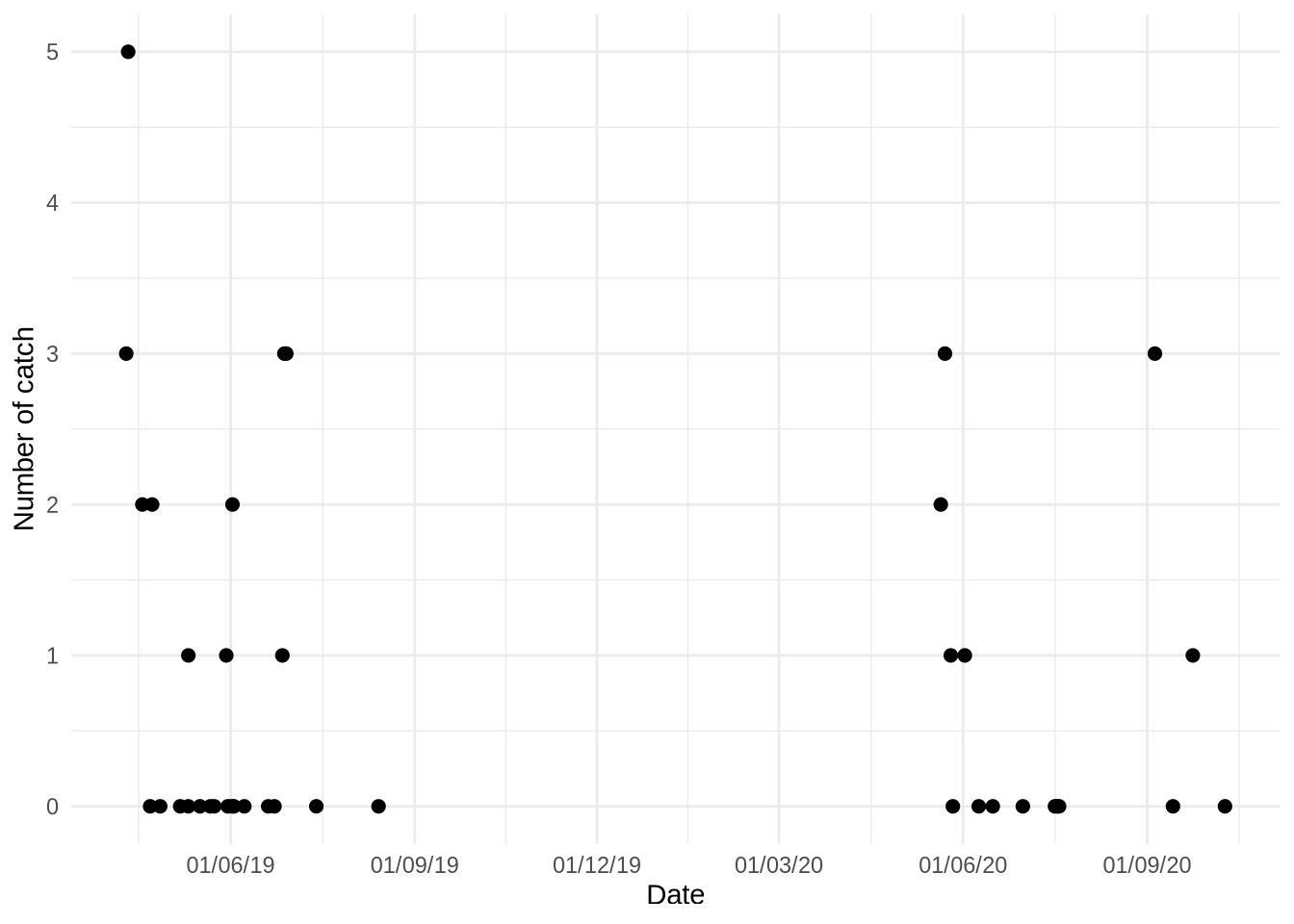
From this graph we see that I didn’t go fishing during the autumn and winter of 2019, I don’t have any data. Unfortunately for me, autumn is known to be a great period for sea bass fishing, I must go fishing this year to compensate the lack of data in this season. During winter, fishing is really complicated because the large majority of sea bass are returned to the ocean.
This graph shows the number of fish I catch depending on the hour of the day :
catch_cond %>%
group_by(Session, Time_beg, .drop = F) %>%
na.omit() %>%
summarise(n_catch = n()) %>%
right_join(unique(catch_cond[, c("Session", "Time_beg")])) %>%
mutate(n_catch = ifelse(is.na(n_catch), 0, n_catch ),
hour = format(Time_beg, "%H")) %>%
ggplot(aes(y = n_catch, x =hour)) +
geom_point( size = 2)  + labs(x = "Hour", y = "Number of catch")+
theme_minimal()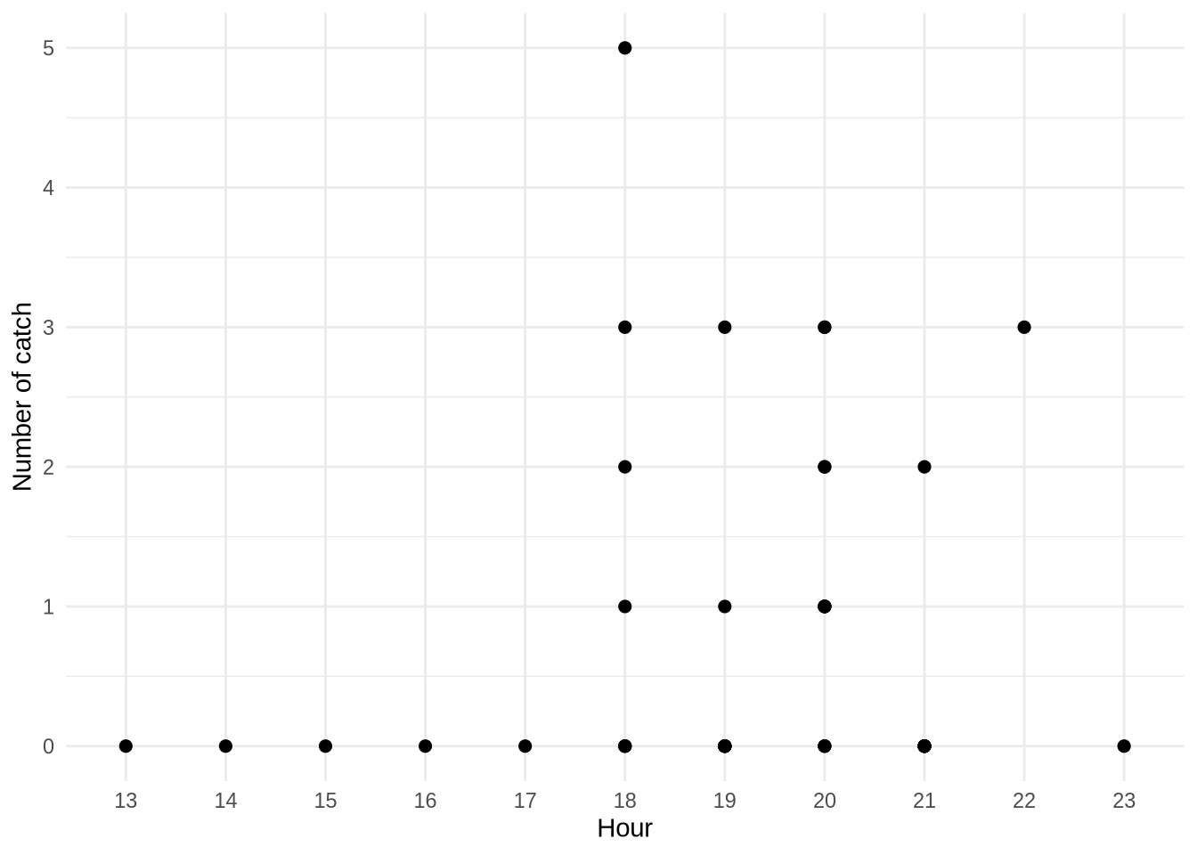
I mostly fish after work or during evenings. To draw relevant conclusions about the influence of the fishing hour, I have to go fishing at different hours of the day (in the morning for example).
The tide is an important parameter for fishing in estuaries. Let’s see the effect of the tide current on my catches:
library(ggpubr)

gg1 <- catch_cond %>%
  group_by(Session, Tide_status_ses, .drop = F)  %>%
  drop_na() %>%
  summarise(n_catch = n()) %>%
  right_join(unique(catch_cond[, c("Session", "Tide_status_ses")])) %>%
  mutate(n_catch = ifelse(is.na(n_catch), 0, n_catch )) %>%
  ggplot(aes(y = n_catch, x = Tide_status_ses, fill = Tide_status_ses)) +
  geom_boxplot() +
  labs(x = "Status of tide current", y = "Number of catch") +
  theme_minimal()+ theme(legend.position="None")

gg2 <- catch_cond %>%
  na.omit() %>%
  ggplot(aes(y = length,x = Tide_status_ses, fill = Tide_status_ses)) +
  geom_boxplot()+
  labs(x = "Status of tide current", y = "Length of the fish") +
  theme_minimal()+ theme(legend.position="None")

ggarrange(gg1, gg2)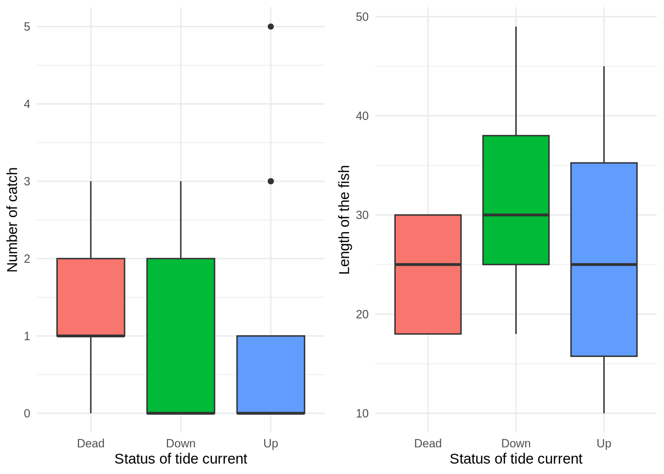
It seems that the status of the tide current does not influence the number of my catch but influences the length of the fish. I tend to catch bigger fish when the current is going down.
A widespread belief among fishermen is that the moon influences greatly the behavior of the fish. Data about the moon phase were available thanks to the weather API, I decided to record this variable to investigate if the belief was true. The two graphs show the number and length of fish depending on the phase of moon (0 corresponding to new moon and 1 to full moon):
gg3 <- catch_cond %>%
  group_by(Session, Moon, .drop = F) %>%
  na.omit() %>%
  summarise(n_catch = n()) %>%
  right_join(unique(catch_cond[, c("Session", "Moon")])) %>%
  mutate(n_catch = ifelse(is.na(n_catch), 0, n_catch )) %>%
  ggplot(aes(y = n_catch, x = Moon)) +
  geom_point( size = 2) +
  labs(x = "Moon phase", y = "Number of catch")+
  theme_minimal()

gg4 <- catch_cond %>%
  ggplot(aes(y = length, x = Moon)) +
  geom_point( size = 2) +
  geom_smooth(method="lm", se=T) +
  labs(x = "Moon phase", y = "Length of the fish")+
  theme_minimal()

ggarrange(gg3, gg4)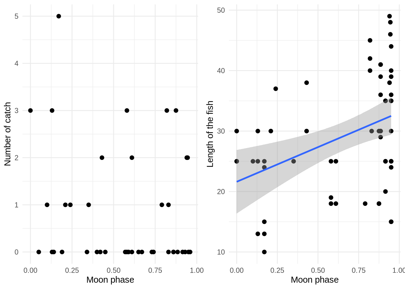
The phase of the moon does not seem to influence the number of fish I catch during a session. However, I tend to catch bigger fish the closer we are to the full moon. To confirm this observation, I need to keep going fishing to get more data !
We can look at the number of fish caught during different weather conditions:
# precipitation probability

gg5 <- catch_cond %>%
  group_by(Session, Preci_prob, .drop = F) %>%
  na.omit() %>%
  summarise(n_catch = n()) %>%
  right_join(unique(catch_cond[, c("Session", "Preci_prob")])) %>%
  mutate(n_catch = ifelse(is.na(n_catch), 0, n_catch )) %>%
  ggplot(aes(y = n_catch, x = Preci_prob)) +
  geom_point()+
  labs(x = "Precipitation prob.", y = "Number of catch")+
  theme_minimal()

# Atm pressure

gg6 <- catch_cond %>%
  group_by(Session, Atm_pres, .drop = F) %>%
  na.omit() %>%
  summarise(n_catch = n()) %>%
  right_join(unique(catch_cond[, c("Session", "Atm_pres")])) %>%
  mutate(n_catch = ifelse(is.na(n_catch), 0, n_catch )) %>%
  ggplot(aes(y = n_catch, x = Atm_pres)) +
  geom_point() +
  labs(x = "Atm. pressure", y = "Number of catch")+
  theme_minimal()

#Air temp

gg7 <- catch_cond %>%
  group_by(Session, Air_temp, .drop = F) %>%
  na.omit() %>%
  summarise(n_catch = n()) %>%
  right_join(unique(catch_cond[, c("Session", "Air_temp")])) %>%
  mutate(n_catch = ifelse(is.na(n_catch), 0, n_catch )) %>%
  ggplot(aes(y = n_catch, x = Air_temp)) +
  geom_point() +
  labs(x = "Air temp.", y = "Number of catch")+
  theme_minimal()


#Cloud cover

gg8 <- catch_cond %>%
  group_by(Session, Cloud_cover, .drop = F) %>%
  na.omit() %>%
  summarise(n_catch = n()) %>%
  right_join(unique(catch_cond[, c("Session", "Cloud_cover")])) %>%
  mutate(n_catch = ifelse(is.na(n_catch), 0, n_catch )) %>%
  ggplot(aes(y = n_catch, x = Cloud_cover)) +
  geom_point() +
  labs(x = "Cloud cover", y = "Number of catchh")+
  theme_minimal()

ggarrange(gg5, gg6, gg7, gg8)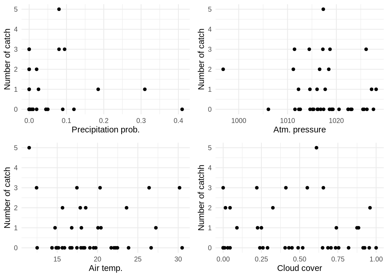
And to their length :
gg15 <- catch_cond %>%
  ggplot(aes(y = length, x = Preci_prob)) +
  geom_point( size = 2) +
  labs( y = "Length of the fish")+
  theme_minimal()

gg16 <- catch_cond %>%
  ggplot(aes(y = length, x = Atm_pres)) +
  geom_point( size = 2) +
  labs( y = "Length of the fish")+
  theme_minimal()

gg17 <- catch_cond %>%
  ggplot(aes(y = length, x = Air_temp)) +
  geom_point( size = 2) +
  labs( y = "Length of the fish")+
  theme_minimal()


gg18  <- catch_cond %>%
  ggplot(aes(y = length, x = Cloud_cover)) +
  geom_point( size = 2) +
  labs( y = "Length of the fish")+
  theme_minimal()

ggarrange(gg15, gg16, gg17, gg18)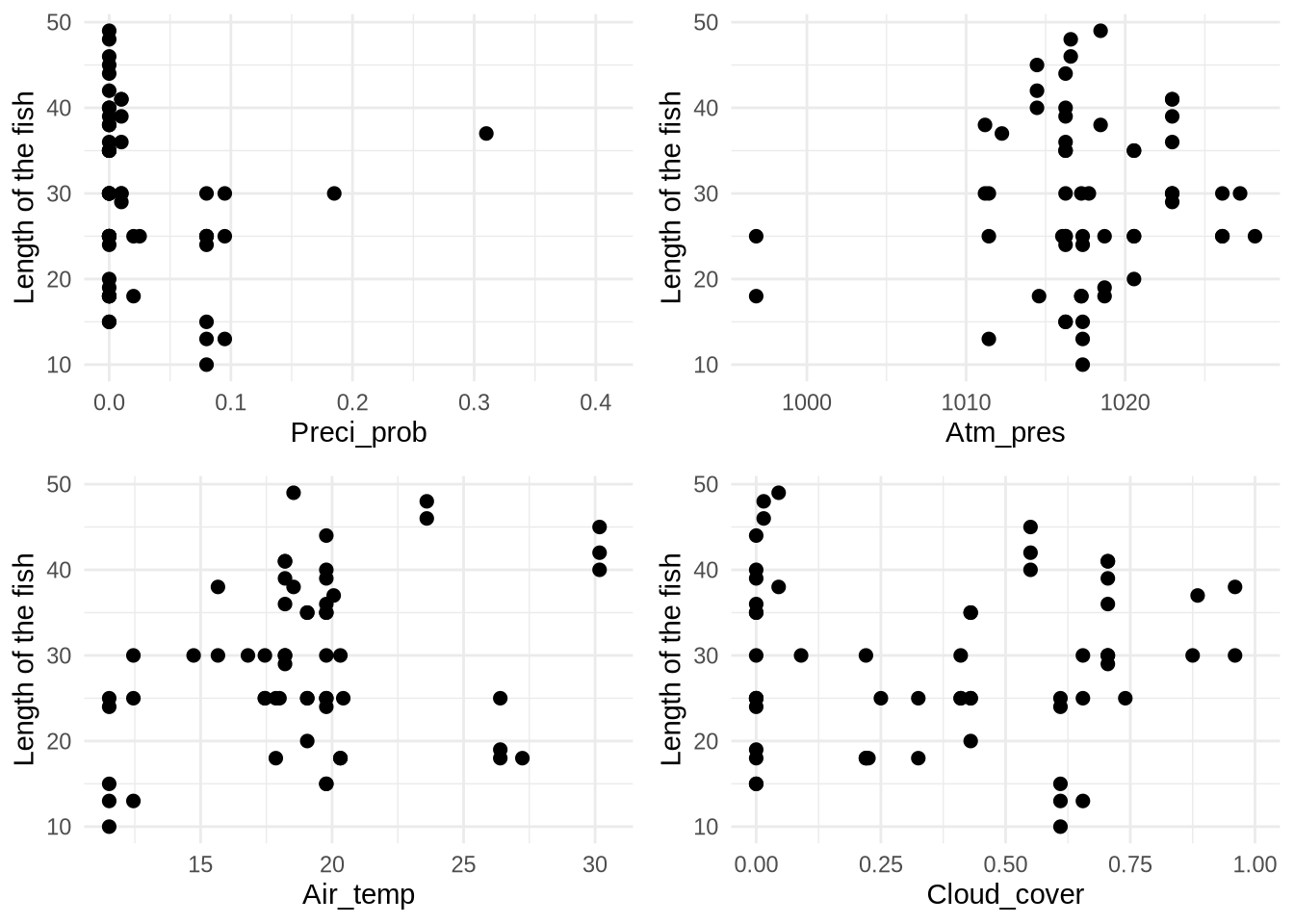
Because we have limited data and not all weather conditions are covered, it is difficult to draw any conclusions.
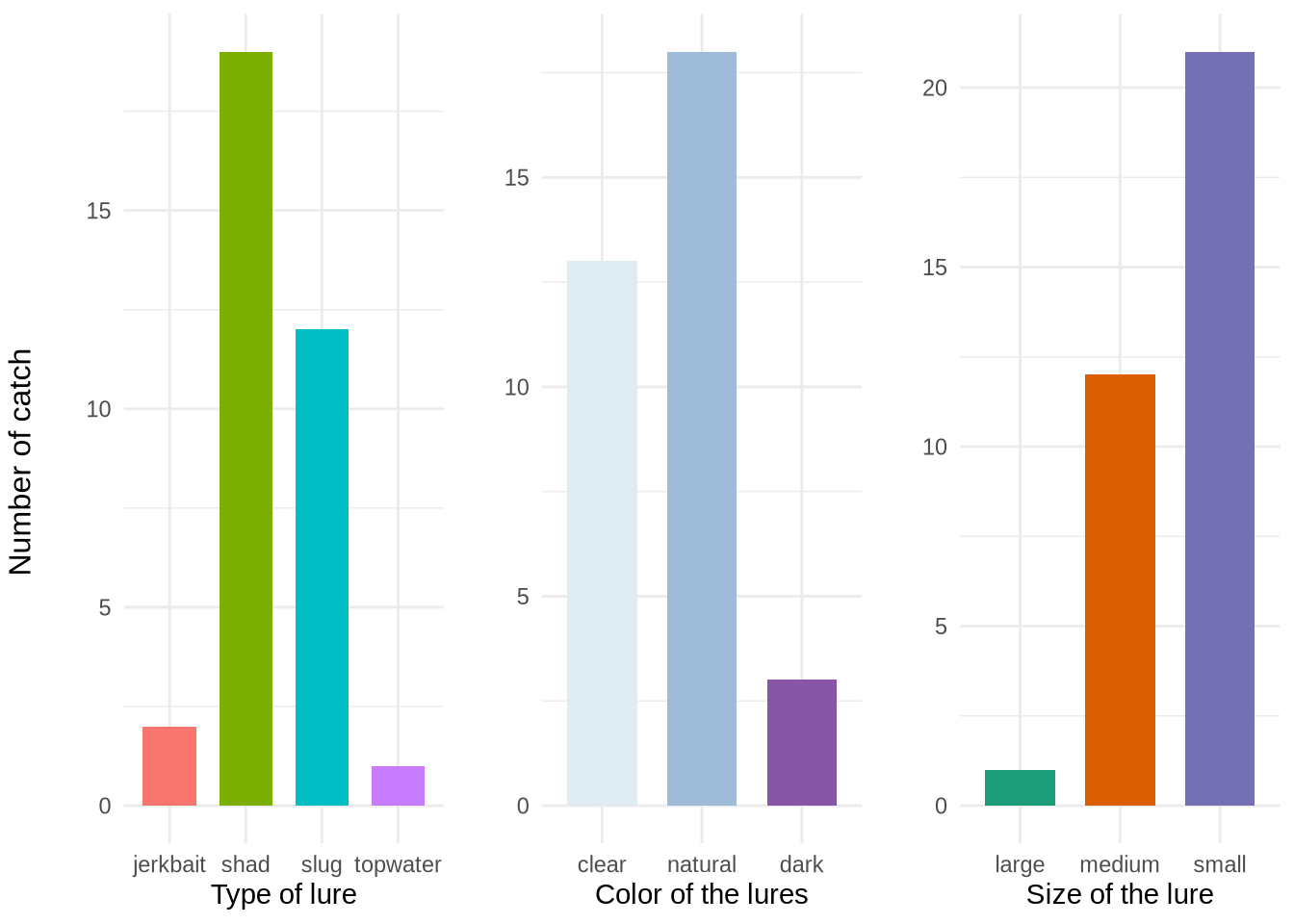
Each time I catch a fish, I fill a form with my shiny application in order to record the characteristics of the lure used. There are different types of lures that have specific swimming patterns, different colors and size. We can represent the number of fish caught depending on the lure characteristics:
levels(catch_cond$colour) <- c("clear", "natural", "dark")
levels(catch_cond$length_lure) <- c("large", "medium", "small")

gg9 <- catch_cond %>%
  na.omit() %>%
  ggplot( aes(x=lure, fill = lure)) +
  geom_bar(stat="count", width=0.7)+
  labs(x = "Type of lure", y = "")+
  theme_minimal()+
  theme(legend.position="None")

gg10 <- catch_cond %>%
  na.omit() %>%
  ggplot( aes(x=colour, fill = colour)) +
  geom_bar(stat="count", width=0.7)+
  labs(x = "Color of the lures", y = "")+
  theme_minimal()+
    scale_fill_brewer(palette="BuPu")+
  theme(legend.position="None")

gg11 <- catch_cond %>%
  na.omit() %>%
  ggplot( aes(x=length_lure, fill = length_lure)) +
  geom_bar(stat="count", width=0.7)+
  labs(x = "Size of the lure", y = "")+
    scale_fill_brewer(palette="Dark2")+
  theme_minimal()+ theme(legend.position="None")

annotate_figure(ggarrange(gg9, gg10, gg11, ncol = 3),
                left = text_grob("Number of catch", rot = 90)
)
We can do the same for the length of fish caught:
gg12 <-catch_cond %>%
  na.omit() %>%
  ggplot(aes(y = length, x = lure, fill=lure)) +
  geom_boxplot()+
  labs(x = "Type of lure", y = "")+
  theme_minimal()+ theme(legend.position="None")

gg13 <-catch_cond %>%
  na.omit() %>%
  ggplot(aes(y = length, x = colour, fill= colour)) +
  geom_boxplot()+
  labs(x = "Color of the lures", y = "")+
  theme_minimal()+
    scale_fill_brewer(palette="BuPu")+ theme(legend.position="None")

gg14 <-catch_cond %>%
  na.omit() %>%
  ggplot(aes(y = length, x = length_lure, fill=length_lure)) +
  geom_boxplot()+
  labs(x = "Size of the lure", y = "")+
  theme_minimal()+
    scale_fill_brewer(palette="Dark2")+ theme(legend.position="None")

annotate_figure(ggarrange(gg12, gg13, gg14, ncol = 3),
                left = text_grob("Length of fish", rot = 90)
)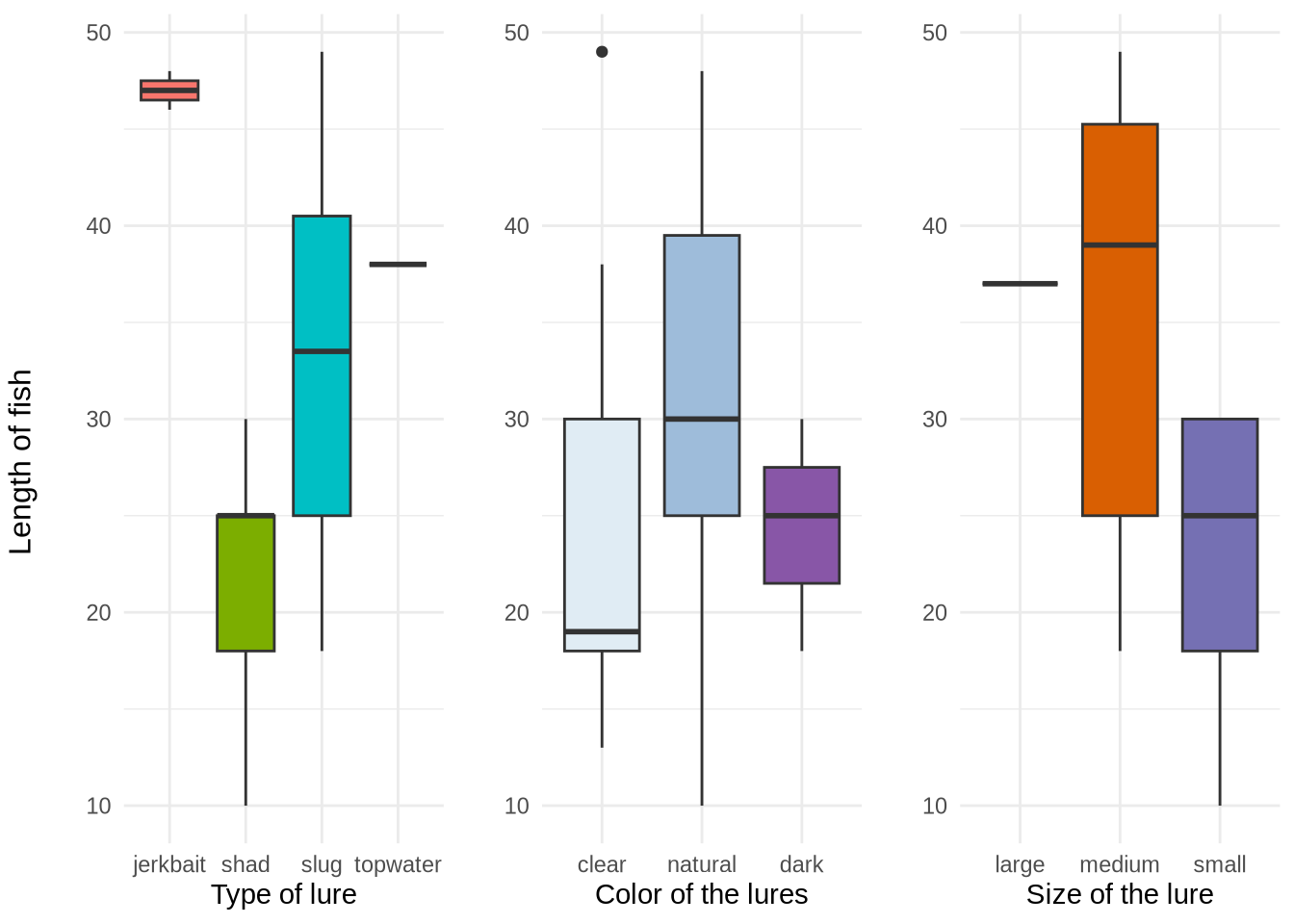
With these 6 graphs, we can see that the most successful types of lures for me are the shad and slug types. An honorable mention is the jerkbait type: it only accounts for 2 fish, but 2 big fish (median around 47cm). The colors that worked best for me were clear and natural. For the size of the lure, bigger lures tend to catch bigger fish in average. These conclusions must be taken with a grain of salt because we do not know the time spent with each lure before catching a fish. In addition, I tend to use the same types and colors of lures (habits), I should vary more.
Analyzing my fishing data was very interesting and it brought me some insights on my fishing style! I understood that I was fishing almost the same way with the same habits. Although it seems to be working for me, I have a biased view on how to catch European sea bass. I must use bigger lures to catch bigger fish and I must vary the types of lures used. Indeed, I fish most of the times with slug or shad lures, hence the higher number of fish caught with these types of lures.
I will keep using the application to gather more data and have a better understanding on my fishing session. I will keep you updated on the results ! :wink: