# General
library(tidyverse)
# Webscraping
library(rvest)
library(RSelenium)
# Geo data
library(tidygeocoder)
library(leaflet)
library(rnaturalearth)
library(sf)
# NLP
library(udpipe)
library(textrank)
library(wordcloud)
# Cleaning
library(stringr)
# Additional functions presented at the end of the post
source('scraping_functions.R') A few weeks ago, I started looking for a data scientist position in industry. My first moves were:
- To look at the job posts on websites such as Indeed
- To update my resume
After reading numerous job posts and work several hours on my resume, I wondered if I could optimize these steps with R and Data Science. I therefore decided to scrape Indeed and analyze the data about data science jobs to:
- Get a visual overview of essential information such as location, type of contract, salary range for the large number of job posts
- Optimize my resume for ATS scan with accurate key words
Loading libraries
The first step is to import several packages:
Collect the data with web scraping
In the beginning of this project, I was using read_html() from rvest to access and download the webpage from Indeed. However, Indeed pages are protected by an anti-scrapping software that blocked any of my requests even though scraping is not forbidden on the pages I am interested in (I checked the robots.txt page).
This is why I decided to access the pages with Rselenium which allows to run an headless browser. We first navigate to the page corresponding to the search results of data scientist jobs in France:
url = "https://fr.indeed.com/jobs?q=data%20scientist&l=France&from=searchOnHP"

# Headless Firefox browser
exCap <- list("moz:firefoxOptions" = list(args = list('--headless')))
rD <- rsDriver(browser = "firefox", extraCapabilities = exCap, port=1111L,
                verbose = F)
remDr <- rD$client

# Navigate to the url
remDr$navigate(url)

# Store page source
web_page <- remDr$getPageSource(header = TRUE)[[1]] %>% read_html()
To scrape a specific information on a webpage you need to follow these steps:
- Find on the web page the element/text/data you want to scrape
- Find the associated xpath or css selector with the developer tool of chrome or firefox ( tutorial here ! )
- Extract the element with
hmtl_element()by indicating the xpath or css selector - Transform the data to text with
html_text2() - Clean the data if necessary
Here is the example with the number of listed data science jobs in France:
web_page %>%
  html_element(css = "div.jobsearch-JobCountAndSortPane-jobCount") %>% # selecting with css
  html_text2() %>% # Transform to text
  str_remove_all("[^0-9.-]") %>% # Clean the data to only get numbers
  substr(start = 2, stop = 8) %>%
  as.numeric()
For now, we can only scrape the data from the first page. However, I am interested in all the job posts and I need to access the other pages ! After navigating through the first 3 pages of listed jobs, I remarked a pattern in the URL address (valid at the time of writing), this means that with a line of code, I can produce a list containing the URLs for the first 40 pages.
Once I have the list, the only thing left is to loop over all the URLs with some delay (good practice for web-scraping), collect the data and clean it with custom functions (at the end of the post):
# Creating URL link corresponding to the first 40 pages
base_url = "https://fr.indeed.com/jobs?q=data%20scientist&l=France&start="
url_list <- c(url, paste0(base_url, as.character(seq(from=10, to=400, by=10))))

# Looping through the URL list
res <- list()
for(i in 1:length(url_list)){
  # Navigate to the URL
  remDr$navigate(url_list[i])

  # Store page source
  web_page <- remDr$getPageSource(header = TRUE)[[1]] %>% read_html()

  # Job title
  job_title <- web_page %>%
    html_elements(css = ".mosaic-provider-jobcards .result") %>%
    html_elements(css = ".resultContent") %>%
    html_element("h2") %>%
    html_text2() %>%
    str_replace(".css.*;\\}", "")

  # URL for job post
  job_url <- web_page %>%
    html_elements(css = ".mosaic-provider-jobcards .result")%>%
    html_elements(css = ".resultContent") %>%
    html_element("h2") %>%
    html_element("a") %>%
    html_attr('href') %>%
    lapply(function(x){paste0("https://fr.indeed.com", x)}) %>%
    unlist()

  # Data about company
  company_info <- web_page %>%
    html_elements(css = ".mosaic-provider-jobcards .result")%>%
    html_elements(css = ".resultContent")%>%
    html_element(css = ".company_location")%>%
    html_text2() %>%
    lapply(FUN = tidy_comploc) %>% # Function to clean the textual data
    do.call(rbind, .)

  # Data about job description
  job_desc <- web_page %>%
    html_elements(css = ".mosaic-provider-jobcards .result")%>%
    html_element(css =".slider_container .jobCardShelfContainer")%>%
    html_text2() %>%
    tidy_job_desc() # Function to clean the textual data related to job desc.

  # Data about salary (when indicated)
  salary_hour <- web_page %>%
    html_elements(css = ".mosaic-provider-jobcards .result .resultContent")%>%
    html_element(css = ".salaryOnly") %>%
    html_text2() %>%
    lapply(FUN = tidy_salary) %>% # Function to clean the data related to salary
    do.call(rbind, .)

  # Job posts in the same format
  final_df <- cbind(job_title, company_info, salary_hour, job_desc, job_url)
  colnames(final_df) <- c("Job_title", "Company", "Location", "Rating", "Low_salary", "High_salary", "Contract_info", "Job_desc", "url")
  res[[i]] <- final_df

  # Sleep 5 seconds, good practice for web scraping
  Sys.sleep(5)
}

# Gather all the job post in a tibble
final_df <- as_tibble(do.call("rbind", res))

# Final data cleaning
final_df <- final_df %>%
  mutate_at(c("Rating", "Low_salary", "High_salary"), as.numeric)

# Clean job title
final_df$Job_title_c <- clean_job_title(final_df$Job_title)
final_df$Job_title_c <- as.factor(final_df$Job_title_c)
We have now a tidy data set! Here is a truncated example of the 5 first rows:
| Job_title | Company | Location | Rating | Low_salary | High_salary | Contract_info | Job_desc | Job_type | Job_title_c |
|---|---|---|---|---|---|---|---|---|---|
| Data Scientist junior (H/F) | Kea & Partners | 92240 Malakoff | NA | 3750 | 4583 | CDI +2 | Travail en journée +1 | Plusieurs postes à pourvoirMaitrise de Python et des packages de data science. 1er cabinet européen de conseil en stratégie à devenir Société à Mission, certifiés B-Corp depuis 2021*,… | Présentiel | data scientist junior |
| Data Scientist (F ou H) | SNCF | Saint-Denis (93) | 3.9 | NA | NA | CDI | Le développement informatique (C, C++, Python, Azure, …). Valider et recetter les phases des projets. Travailler avec des méthodes agiles avec les équipes et… | Présentiel | data scientist |
| Data Scientist (H/F) (IT) | Yzee Services | Paris (75) | 3.3 | 2916 | 3750 | Temps plein | Recueillir, structurer et analyser les données pertinentes pour l'entreprise (activité liée à la relation client, conseil en externe). | Présentiel | data scientist |
| Data Scientist H/F | Natan (SSII) | Paris (75) | NA | 4583 | 5833 | CDI +1 | Travail en journée | Plusieurs postes à pourvoirVous retrouverez une *ESN ambitieuse portée par le goût de l’excellence.*. Au sein du département en charge d'automatisation transverse des besoins de la… | Présentiel | data scientist |
| Data Scientist Junior H/F / Freelance | karma partners | Roissy-en-Brie (77) | NA | 400 | 550 | Temps plein +1 | Le profil recherché est un profil junior (0-2 ans d'expérience) en data science, avec une appétence technique et des notions d'architecture logicielle et de… | Présentiel | data scientist junior |
Visualization of the proposed salaries
Let’s see if we can get some insights about data science jobs by making some graphical representations. The first thing I wanted to know is how much the companies are willing to pay in order to recruit a data science candidate. I therefore decided to make some figures about the salary range depending on the company and the job title.
Beware!
The following graphs must be taken with a grain of salt as they display a small sample of the data. Indeed, the salary was listed for only 14% of the job post. The insights or trends in these graphs may not be representative of companies that have not listed their proposed salary.
Salary by company
The following graphic shows the monthly income listed by some companies (not all the companies list their proposed salary):
# Function to make euro X scale
euro <- scales::label_dollar(
  prefix = "",
  suffix = "\u20ac",
  big.mark = ".",
  decimal.mark = ","
)

final_df %>%
  filter(Low_salary > 1600) %>% # To remove internships and freelance works
  select(Company, Low_salary, High_salary) %>%
  group_by(Company) %>%
  summarize_if(is.numeric, mean) %>%
  mutate(Mean_salary = rowMeans(cbind(Low_salary, High_salary), na.rm = T),
           Company = fct_reorder(Company, desc(-Mean_salary))) %>%
  ggplot(aes(x = Company)) +
  geom_point(aes(y = Mean_salary), colour = "#267266") +
  geom_linerange(aes(ymin = Low_salary, ymax = High_salary)) +
  geom_hline(aes(yintercept = median(Mean_salary)), lty=2, col='red', alpha = 0.7) +
  scale_y_continuous(labels = euro) +
  ylab("Monthly income") +
  xlab("") +
  coord_flip() +
  theme_bw(base_size = 8)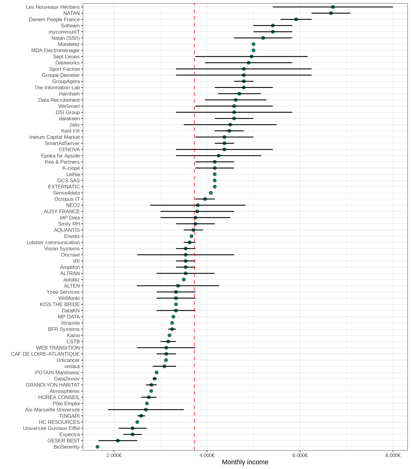
The median monthly salary is around 3700 euros. As you can see the salaries can vary a lot depending on the company. This is partly due because I didn’t make distinction between the different data science jobs (data scientist, data analyst, data engineer, senior or lead).
Salary by job title
We can plot the same graph but instead of grouping by company we can group by job title:
final_df %>%
  filter(Low_salary > 1600) %>%  # To remove internships and freelance works
  select(Job_title_c, Low_salary, High_salary, Job_type) %>%
  group_by(Job_title_c) %>%
  summarize_if(is.numeric, ~ mean(.x, na.rm = TRUE)) %>%
  mutate(Mean_salary = rowMeans(cbind(Low_salary, High_salary), na.rm = T),
         Job_title_c = fct_reorder(Job_title_c, desc(-Mean_salary))) %>%
  ggplot(aes(x = Job_title_c, y = Mean_salary)) +
  geom_point(aes(y = Mean_salary), colour = "#267266") +
  geom_linerange(aes(ymin = Low_salary, ymax = High_salary)) +
  #geom_label(aes(label = n, Job_title_c, y = 1500), data = count_df) +
  scale_y_continuous(labels = euro) +
  theme_bw(base_size = 12) +
  xlab("") +
  ylab("Monthly Income") +
  coord_flip()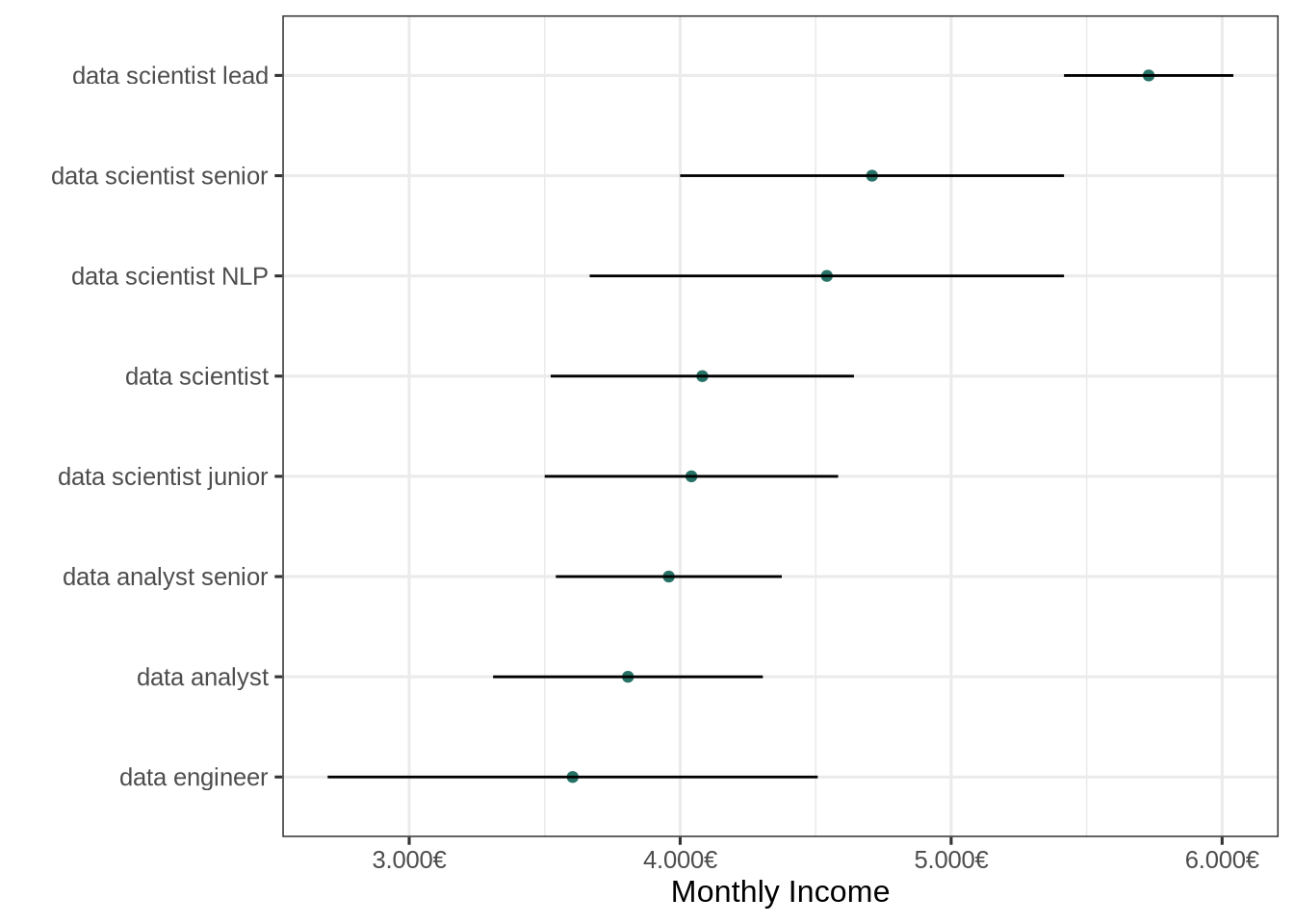
We clearly see the differences in proposed salaries depending on the job title: data scientists seem to earn slightly more in average than data analysts. The companies also seem to propose higher salaries for jobs with more responsibilities or requiring more experiences (senior, lead).
Salary depending on location: full remote, hybrid, on site ?
Finally we can plot the salaries depending on the location (full remote, hybrid, on site) to see if it has an impact:
# Tidy the types and locations of listed jobs
final_df <- tidy_location(final_df)
count_df <- count(final_df %>% filter(Low_salary > 1600), Job_type)
final_df %>%
  filter(Low_salary > 1600) %>%
  drop_na(Location) %>%
  mutate(Mean_salary = rowMeans(cbind(Low_salary, High_salary), na.rm = T),
         Job_type = as.factor(Job_type)) %>%
    ggplot(aes(x = Job_type, y = Mean_salary)) +
  geom_boxplot(na.rm = TRUE) +
  geom_label(aes(label = n, Job_type, y = 5500), data = count_df) +
  scale_y_continuous(labels = euro) +
  theme_bw(base_size = 12) +
  xlab("Job Type") +
  ylab("Income")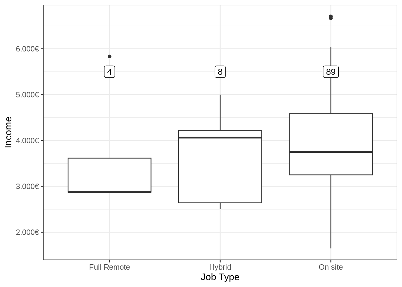
It is worth noting that most of the jobs proposed in France are on site jobs. The median salary for this type of jobs is slightly lower than hybrid jobs. The salary distribution of full remote and hybrid jobs must be taken with care as it is only represented by 12 job posts.
Mapping job locations
During my job search, I was frustrated not to see a geographical map regrouping the locations of all the proposed jobs. Such map could help me greatly in my search. Let’s do it !
First, we must tidy and homogenize the locations for all the job posts. To this end, I made a custom function (tidy_location()) which includes some stringr functions, you can find more details about this function at the end of this post. It outputs the location in this format [Town]([Zip code]). Even though all the locations have been homogenized, it can not be plotted on a map (we need the longitude and latitude). To get the latitude and longitude with the town name and zip code I used the geocode() function from tidygeocoder package.
# Extract coordinates from town name
final_df <- final_df %>%
  mutate(Loc_tidy_fr = paste(Loc_tidy, 'France')) %>%
  geocode(Loc_tidy_fr, method = 'arcgis', lat = latitude , long = longitude) %>%
  select(- Loc_tidy_fr)
Distribution of Data Science jobs in France
We can now represent the number of Data Science jobs by departments:
# Map of France from rnaturalearth package
france <- ne_states(country = "France", returnclass = "sf") %>%
  filter(!name %in% c("Guyane française", "Martinique", "Guadeloupe", "La Réunion", "Mayotte"))

# Transform location to st point
test <- st_sf(final_df, geom= lapply(1:nrow(final_df), function(x){st_point(c(final_df$longitude[x],final_df$latitude[x]))}))
st_crs(test) <- 4326

# St_join by departments
joined <- france %>%
  st_join(test, left = T)

# Custom breaks for visual representation
my_breaks = c(0, 2, 5, 10, 30, 50, 100, 260)

joined %>%
  mutate(region=as.factor(name)) %>%
  group_by(region) %>%
  summarize(Job_number=n()) %>%
  mutate(Job_number = cut(Job_number, my_breaks)) %>%
  ggplot() +
  geom_sf(aes(fill=Job_number), col='grey', lwd=0.2) +
  scale_fill_brewer("Job number",palette = "GnBu") +
  theme_bw()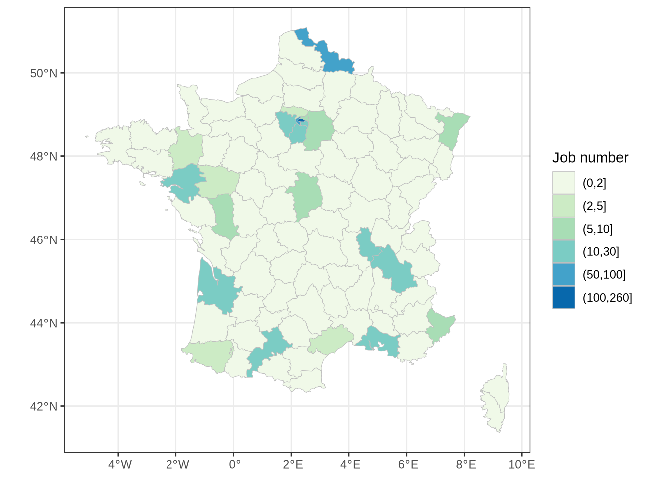
It is really interesting to see that the distribution of jobs is quite heterogeneous in France. The majority of the jobs are concentrated in a few departments that include a large city. It is expected as most of the jobs are proposed by large company that are often installed in the proximity of important cities.
Interactive map
We can go further and plot an interactive map with leaflet which allows us to search dynamically for a job post:
# Plot leaflet map
final_df %>%
  mutate(pop_up_text = sprintf("<b>%s</b> <br/> %s",
                                     Job_title, Company)) %>% # Make popup text
  leaflet() %>%
  setView(lng = 2.36, lat = 46.31, zoom = 5.2) %>% # Center of France
  addProviderTiles(providers$CartoDB.Positron) %>%
  addMarkers(
    popup = ~as.character(pop_up_text),
    clusterOptions = markerClusterOptions()
  )
Analyzing job descriptions
Nowadays most of the resumes are scanned and interpreted by an applicant tracking system (ATS). To make things simple, this system looks for key words in your resume and assess the match with the job you are applying for. It is therefore important to describe your experiences with specific key words to improve the chances of getting to the next step of the hiring process.
But what key words should I include in my resume ? Let’s answer this question by analyzing the job descriptions of data scientist jobs.
Downloading and cleaning each job description
First we download the full description of each job by navigating through all the URL listed in our table. We then clean and homogenize the description with a custom function:
# Loop through all the URLs
job_descriptions <- list()
pb <- txtProgressBar(min = 1, max = length(final_df$url), style = 3)
for(i in 1:length(final_df$url)){
  remDr$navigate(final_df$url[i])
  web_page <- remDr$getPageSource(header = TRUE)[[1]] %>% read_html()
  job_descriptions[[i]] <- web_page %>%
        html_elements(css = ".jobsearch-JobComponent-description") %>%
      html_text2()
  Sys.sleep(2)
  setTxtProgressBar(pb, i)
}
# Gathering in dataframe
job_descriptions <- as.data.frame(do.call("rbind", job_descriptions))
names(job_descriptions) <- c("Description")

# Binding to same table:
final_df <- cbind(final_df, job_descriptions)

# Homogenize with custom function
final_df$Description_c <- lapply(final_df$Description, function(x){clean_job_desc(x)[[2]]})
final_df$Language <- textcat::textcat(final_df$Description)
Annotation procedure with udpipe Package
This part is inspired from this post.
Now that the descriptions of all the listed jobs are imported and pre-cleaned, we can annotate the textual data with udpipe package. This package contains functions and models which can perform tokenisation, lemmatisation and key word extraction.
We first restrict this analysis to data scientist job post written in french, then we annotate all the descriptions:
# Restricting the analysis to Data scientist post written in french
desc_data_scientist <- final_df %>%
  filter((Job_title_c == "data scientist") & (Language == "french")) %>%
  select(Description_c)

ud_model <- udpipe_download_model(language = "french") # Download the model if necessary
ud_model <- udpipe_load_model(ud_model$file_model)

# Annotate the descriptions
x <- udpipe_annotate(ud_model, x = paste(desc_data_scientist, collapse = " "))
x <- as.data.frame(x)
Most common nouns
We can visualize the most employed word throughout the data scientist job posts written in french:
stats <- subset(x, upos %in% "NOUN")
stats <- txt_freq(x = stats$lemma)

stats %>%
  top_n(50, freq) %>%
  mutate(key = as.factor(key),
         key = fct_reorder(key, freq)) %>%
  ggplot(aes(x = key, y = freq)) +
  geom_bar(stat = 'identity') +
  coord_flip() +
  ylab("Most common nouns") +
  theme_bw()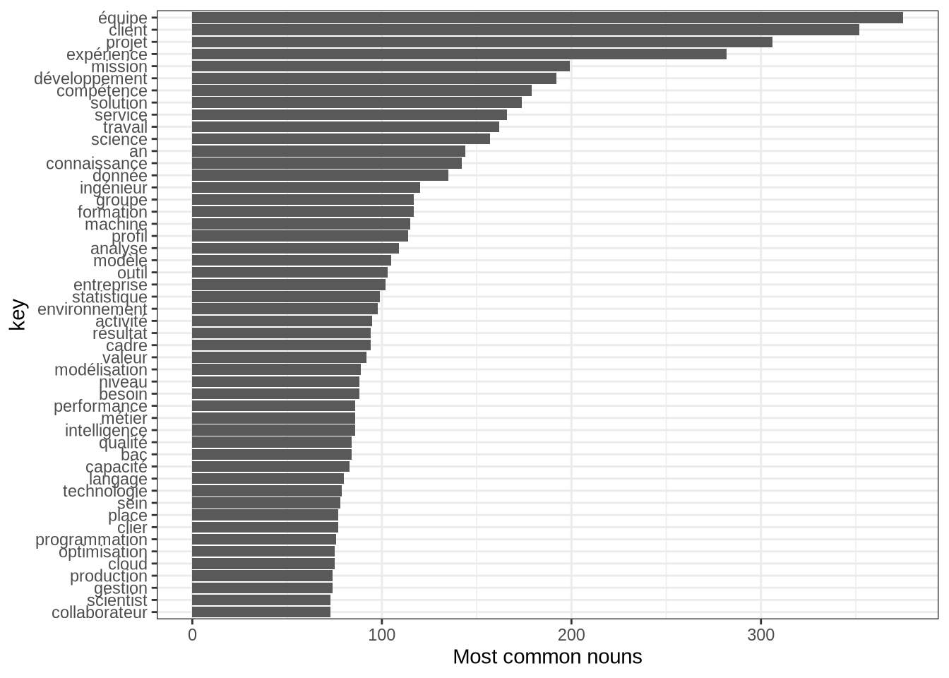
Even though, it gives us an idea of words to include it is not very informative as key words are often composed by two or more words.
Extracting key words for resume writing
There are several methods implemented in udpipe to extract key words from a text. After testing several methods, I selected the Rapid Automatic Keyword Extraction (RAKE) which gives me the best results:
stats <- keywords_rake(x = x,
                       term = "token",# Search on token
                       group = c("doc_id", "sentence_id"), # On every post
                       relevant = x$upos %in% c("NOUN", "ADJ"),  # Only among noun and adj.
                       ngram_max = 2, n_min = 2, sep = " ")

stats <- subset(stats, stats$freq >= 5 & stats$rake > 3)

stats %>%
  arrange(desc(rake)) %>%
  head()
keyword ngram freq rake
1 intelligence artificielle 2 9 9.368889
2 tableaux bord 2 5 8.504274
3 formation supérieure 2 5 8.374725
4 modèles prédictifs 2 15 7.581294
5 force proposition 2 6 7.190238
6 production échelle 2 5 7.034038wordcloud(words = stats$keyword, freq = stats$freq, min.freq = 3,
max.words=100, random.order=FALSE, rot.per=0.35,
colors=brewer.pal(8, "Dark2"), scale = c(2.5, .5))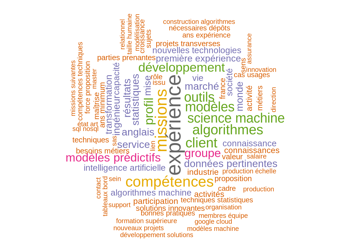
We can see that this method has selected important french key words related to the data scientist job ! In the first positions, we find the key words: “artificial intelligence”, “dashboards”, “higher education”, “predictive model”. I’d better check if these words appear on my resume !
Conclusion
I hope I convinced you that it is possible to optimize your job search with Data Science!
If this post has caught your interest and you are looking for a new Data Scientist, do not hesitate to contact me on my mail as I am currently looking for a job in France (Hybrid, Remote) or in Europe (Remote).
Custom functions to clean data extracted from the webpage
These functions use several methods such as regular expressions, stop words and conditional statements to clean the textual data.
library(rvest)
library(stringr)
library(httr)
library(tidystopwords)
library(textcat)

# Function to tidy the data related to the company
tidy_comploc <- function(text){
  lst <- str_split(text, pattern = "\n", simplify =T)
  ext_str <- substr(lst[1], nchar(lst[1])-2, nchar(lst[1]))
  res <- suppressWarnings(as.numeric(gsub(',', '.', ext_str)))
  lst[1] <- ifelse(is.na(res), lst[1], substr(lst[1], 1, nchar(lst[1])-3))
  lst[3] <- res
  t(as.matrix(lst))
}

# Function to tidy the short job description provided with the job post
tidy_job_desc <- function(text){
  stopwords <- c("Candidature facile", "Employeur réactif")
  text <- str_remove_all(text, paste(stopwords, collapse = "|"))
  stopwords_2 <- "(Posted|Employer).*"
  text <- str_remove_all(text, stopwords_2)
  text
}

# Function to tidy the salary data if provided
tidy_salary <- function(text){
  if(is.na(text)){
    others <- NA
    sal_low <- NA
    sal_high <- NA
  }else{
    text <- str_split(text, "\n", simplify = T)
    others <- paste(text[str_detect(text, "€", negate = T)], collapse = " | ")
    sal <- text[str_detect(text, "€", negate = F)]
    if(rlang::is_empty(sal)){
      sal_low <- NA
      sal_high <- NA
    }else{
      range_sal <- as.numeric(str_split(str_remove_all(str_replace(sal, "à", "-"), "[^0-9.-]"), "-", simplify = TRUE))
      sal_low <- sort(range_sal)[1]
      sal_high <- sort(range_sal)[2]

      if(str_detect(sal, "an")){
        sal_low <- floor(sal_low/12)
        sal_high <- floor(sal_high/12)
      }
    }
  }
  return(c(as.numeric(sal_low), as.numeric(sal_high), others))
}

# Function to tidy the location of the job (Remote/Hybrid/Onsite) + homogenize
# location and zip code
tidy_location <- function(final_df){
  final_df$Job_type <- ifelse(final_df$Location == "Télétravail", "Full Remote", ifelse(str_detect(final_df$Location, "Télétravail"), "Hybrid", "On site"))
  final_df$Loc_possibility <- ifelse(str_detect(final_df$Location, "lieu"), "Plusieurs lieux", NA)
  stopwords <- c("Télétravail à", "Télétravail", "à", "hybride")
  final_df$Loc_tidy <- str_remove_all(final_df$Location, paste(stopwords, collapse = "|"))
  final_df$Loc_tidy <- str_remove_all(final_df$Loc_tidy, "[+].*")
  final_df$Loc_tidy <- str_trim(final_df$Loc_tidy)
  final_df$Loc_tidy <-  sapply(final_df$Loc_tidy,
                               function(x){
                                 if(!is.na(suppressWarnings(as.numeric(substr(x, 1, 5))))){
                                   return(paste(substr(x, 7, 30), paste0('(', substr(final_df$Loc_tidy[2], 1, 2), ')')))
                                 }else{
                                   return(x)
                                 }})
  return(final_df)
}

# Function to keep only certain words in text
keep_words <- function(text, keep) {
  words <- strsplit(text, " ")[[1]]
  txt <- paste(words[words %in% keep], collapse = " ")
  return(txt)
}

# Homogenize the job title and class them in a few categories
clean_job_title <- function(job_titles){
  job_titles <- tolower(job_titles)
  job_titles <- gsub("[[:punct:]]", " ", job_titles, perl=TRUE)

  words_to_keep <- c("data", "scientist", "junior", "senior", "engineer", "nlp",
                     "analyst", "analytics", "analytic", "science", "sciences",
                     "computer", "vision", "ingenieur", "données", "analyste",
                     "analyses", "lead", "leader", "dataminer", "mining", "chief",
                     "miner", "analyse", 'head')
  job_titles_c <- unlist(sapply(job_titles, function(x){keep_words(x, words_to_keep)}, USE.NAMES = F))
  job_titles_c <- unlist(sapply(job_titles_c, function(x){paste(unique(unlist(str_split(x, " "))), collapse = " ")}, USE.NAMES = F))
  table(job_titles_c)

  data_analytics_ind <-  job_titles_c %in% c("analyses data", "analyst data", "analyste data", "analyste data scientist", "data analyse",
                                             "analyste données", "analytic data scientist", "analytics data", "analytics data engineer", "data analyst engineer",
                                             "data analyst données", "data analyst scientist", "data analyst scientist données", "data analyste", "data analyst analytics",
                                             "data analytics", "data analytics engineer", "data engineer analyst", "data scientist analyst", "data scientist analytics")
  job_titles_c[data_analytics_ind] <- "data analyst"

  data_analytics_j_ind <-  job_titles_c %in% c("junior data analyst", "junior data analytics", "junior data scientist analyst")
  job_titles_c[data_analytics_j_ind] <- "data analyst junior"

  data_scientist_ind <- job_titles_c %in% c("data computer science", "data science", "data science scientist", "data sciences",
                                            "data sciences scientist", "data scientist données", "data scientist sciences",
                                            "données data scientist", "scientist data", "science données", "scientist data",
                                            "scientist data science", "computer data science", "data science données", "data scientist science")
  job_titles_c[data_scientist_ind] <- "data scientist"

  data_scientist_j_ind <- job_titles_c %in% c("junior data scientist")
  job_titles_c[data_scientist_j_ind] <- "data scientist junior"

  data_engineer_ind <- job_titles_c %in% c("data engineer scientist", "data science engineer", "data miner", "data scientist engineer",
                                           "dataminer", "engineer data scientist", "senior data scientist engineer", "ingenieur data scientist")
  job_titles_c[data_engineer_ind] <- "data engineer"

  nlp_data_scientist_ind <- job_titles_c %in% c("data scientist nlp", "nlp data science",
                                                "nlp data scientist", "senior data scientist nlp")
  job_titles_c[nlp_data_scientist_ind] <- "data scientist NLP"

  cv_data_scientist_ind <- job_titles_c %in% c("computer vision data scientist", "data science computer vision",
                                               "data scientist computer vision")
  job_titles_c[cv_data_scientist_ind] <- "data scientist CV"

  lead_data_scientist_ind <- job_titles_c %in% c("chief data", "chief data scientist", "data scientist leader", "lead data scientist",
                                                 "data chief scientist", "lead data scientist senior", "head data science")
  job_titles_c[lead_data_scientist_ind] <- "data scientist lead or higher"
  senior_data_scientist_ind <- job_titles_c %in% c("senior data scientist")
  job_titles_c[senior_data_scientist_ind] <- "data scientist senior"

  senior_data_analytics_ind <- job_titles_c %in% c("senior analytics data scientist", "senior data analyst", "senior data scientist analytics")
  job_titles_c[senior_data_analytics_ind] <- "data analyst senior"


  lead_data_analyst_ind <- job_titles_c %in% c("lead data analyst senior", "lead data analyst")
  job_titles_c[lead_data_analyst_ind] <- "data analyst lead"
  return(job_titles_c)
}

# Function to clean the full job description before word annotation
clean_job_desc <- function(text){
  text <- tolower(text)
  text <- str_replace_all(text, "\n", " ")
  text <- str_remove(text, pattern = "dé.*du poste ")
  text <- str_remove(text, pattern = "analyse de recr.*")
  text <- gsub("(?!&)[[:punct:]+’+…+»+«]", " ", text, perl=TRUE)

  language <- textcat(text)

  if(language == "french"){
    text <- str_replace_all(text, "œ", "oe")
    stopwords <- c("détails", "poste", "description", "informations", "complémentaires", "c", generate_stoplist(language = "French"))
  }else{
    stopwords <- c("description", generate_stoplist(language = "English"))
  }

  text <- str_replace_all(text, paste(stopwords, collapse = " | "), " ")
  text <- str_replace_all(text, paste(stopwords, collapse = " | "), " ")
  text <- str_replace_all(text, paste(stopwords, collapse = " | "), " ")

  return(c(language, text))
}